Simply put, to see the greatest return on investing in genomically-enhanced EPDs (GE-EPDs), cattle breeders must decrease the average age of sires and dams. The purpose of this article is to explain why, as well as other contributing factors to the rate of genetic gain.
But first, we must start with an equation, referred to as the “Key Equation” or “Breeders Equation” as follows:
∆G/y = [r * sg * i ] / L
where:
∆G = the change per year in the trait’s genetic merit within the population.
r = the accuracy of the selection.
sg = the amount of genetic variation present in the population.
i = the selection intensity.
L = the generation interval.
While a bit technical at first glance, it becomes more straightforward as each component is broken down.
Accuracy of selection (r) is the correlation between the true breeding value and the estimate used for selection decisions. When observed measurements, such as actual weaning weight, are used to make selection decisions, r is the square root of the heritability (i.e., the portion of variation in the trait due to genetics). When EPDs are used for selection, the accuracy of the EPD determines r. This makes genomic testing of seedstock animals even more paramount as the biggest advantage to the technology is its ability to increased accuracy of a GE-EPD.
The genetic variability of the trait, measured by a standard deviation (sg), within the population represents how much observations range around the average. Using the weaning weight example, this would be how much spread exists between the heaviest and lightest calf at weaning. If most animals are close to average, the standard deviation is small. If there is more spread, or variation, and animals are not as close to average, the standard deviation is larger. In terms of the response to selection (∆G) the amount of genetic variability is the one component that breeders do not typically have as much control as most is driven by biology, specifically Mendelian sampling.
The selection intensity (i) measures how different the selected parents are from the overall population average. This would be the replacement heifers and cows chosen for “next” year’s breeding, as well as bulls, compared to the previous year. If the selected parents are close to the population average, the selection intensity is small. If the parents are quite different from the population average, the selection intensity is large. In other words, the selection intensity reflects whether the parents are from the top 25%, 5%, 1%, etc. of the population (i.e., percentile rank). An easy way to think about this is comparing a herd bull to a sire marketed by a semen company. In most cases, selecting a sire for use via artificial insemination (AI) would lead to a higher selection intensity, and faster rate of genetic gain.
The focus of this fact sheet is changing the generation interval (L). The generation interval is the average age of parents when the next generation is born. If older bulls and cows are used as parents, the generation interval is longer and genetic change is slower. But if we use younger bulls and cows and replace older generations with younger animals, the generation interval shortens and genetic progress is more rapid. This is because we are “turning over” the genetics of the herd, quicker. Mathematically speaking, using the equation presented earlier, L is in the denominator by itself and thus can have a large impact on the amount of genetic progress that can be made.
Effect of decreasing generation interval
Let’s look at some historical data to get a feel for the relationships between selection accuracy, selection intensity, and generation interval. From a study analyzing 3,750 Angus animals, the rate of genetic change from weaning weight was estimated to increase 2.8 pounds per year, with a genetic standard deviation of 26.3 pounds, and a generation interval of 5 years. Plugging these values into the equation above and solving, leaves accuracy multiplied by intensity equaling 0.53 (r*i=0.53). If we assume true accuracy of selection is 0.5 (equal to a BIF accuracy of 0.13), then selection intensity for this population is 1.07.
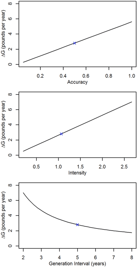
We can vary the values of accuracy, intensity and generation interval and observe the results on genetic change. The graphs in Figure 1 depict that increasing accuracy of selection by 20% results in a 16.7% increase in genetic change, while increasing intensity by 20% results in a 20% increase in genetic change. (The slope of the lines in the top two panels of Figure 1 are not the same.) However, by decreasing generation interval by 20% (5 years to 4 years) we see a 25% increase in genetic change. Further, unlike the relationship between ∆G and r or i, the relationship between ∆G and L is not a straight line; ∆G increases more rapidly as we decrease L. If we decrease generation interval from 5 years to 3.5 years, genetic change increases by 43%. Thus, because generation interval is the lone term in the denominator of the genetic change equation, it has the largest impact on genetic change per year.
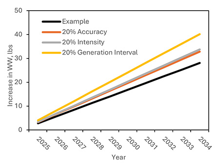
But this genetic change only applies to a single selection year. Each year this builds on top of itself, compounding overtime. Figure 2 shows how genetic change over time would look across 10 years for the initial example of 2.81 lb. per year, compared to a 20% increase in accuracy, selection intensity, and 20% decrease in generation interval. After 10 years, there is a 12.1 lb. difference in weaning weight compared to the initial example.
But there’s more good news. Historically, accuracy and generation interval were not independent. To increase accuracy we needed older bulls with more progeny records, thus generation interval increased. To decrease generation interval, we used younger bulls with less data and lower accuracy. As previously introduced, GE-EPDs can help alleviate this negative relationship by increasing the accuracy of selection on younger, “unproven” animals. For example, depending on the genetic evaluation and trait, adding genomic information on an animal is the equivalent of 8 to 35 progeny records, all before they have their first calf.
Strategies to decrease generation interval
What are some strategies we can use to increase genetic progress by decreasing generation interval while still balancing accuracy and intensity? The bull side of the equation has the easiest identified solutions. We often see beef producers use proven bulls that are 10 or 15 years old in artificial insemination programs. While this may seem a useful practice due to increased EPD accuracy providing confidence particularly for traits like calving ease, the advent of genomic testing helps to mitigate this concern. The article has outlined the immense benefit from using younger sires, all while the risk of which can be offset by using more than one bull. This practice has been successfully employed in the dairy and swine industries for years, due to several advantages. First, using young sires shortens the generation interval and increases genetic progress, as we have previously discussed. Second, young sires take advantage of the genetic trend of a breed, thus they are more likely to rank higher for the economically important traits that are under selection compared to older sires. Third, new developments in genomic testing have increased the accuracy of young sire EPDs. While historically EPD accuracies of young bulls have been around 0.1, GE- EPD accuracies are closer to 0.4 depending upon the trait of interest. Fourth, by using a larger number of sires, producers can hedge against unfavorable changes in EPD estimates. As the EPD estimates for the selected young sires become more accurate with additional new data, some sire’s EPDs will improve whereas the EPDs of other sires will worsen. In this case, the progeny of the under-performing sire can be sold as feeder calves, and the producer will reap the benefits of the sire’s progeny that outperformed his previous EPD estimate. For example, a producer selects a group of bulls that rank in the 15th percentile for an economic selection index. As newly collected data are used in EPD estimation in the following years, some sires will stay near the 15th percentile, some will drop to the 25th percentile and some will rise to the 5th percentile. As a consequence, the average of the bull battery stays intact, and in fact the accuracy of the mean of the group is larger than the accuracy of any one sire. The producer can choose to sell the progeny of bulls that fell to the 25th percentile. But, the producer now has progeny sired by a bull in the 5th percentile, i.e., thus the bull performed better than expected.
Strategies to decrease the generation interval on the female side of the equation may be cost prohibitive. It often takes 5 to 6 years of production for a producer to break even on the investment in a cow in a commercial operation. But the seedstock sector may have opportunities to shorten the generation interval in females. One approach may be to use younger females in embryo transfer programs. With a genomic prediction, cows can have the same accuracy behind their GE-EPDs as if they had 8 to 35 progeny records. These more reliable EPD estimates may allow producers to use younger cows as embryo donors. This approach will not be as dramatic as using younger sires.
Conclusion
When a systematic approach is taken to decrease generation interval by balancing accuracy and intensity, more rapid genetic change can be achieved. The largest gains in accuracy from genomic predictions are seen in young animals with little performance data behind their EPD estimates. By using these young animals as parents we take advantage of the investment in genomic testing, but we also shorten the generation interval. By using a larger number of sires with GE-EPDs we can take advantage of the increased genetic progress resulting from a shorter generation interval.