Technically, various mating schemes of animals are classified under two broad categories — inbreeding and outbreeding. Classification depends on the closeness of the biological relationship between mates. Within each category, a wide variation in intensity of this relationship exists. A very fine line separates the two categories. Mating closely related animals (for example, parent and offspring, full brother and sister or half brother and sister) is inbreeding. With less closely related animals (first cousins, second cousins), people disagree about where to draw the line between inbreeding and outbreeding.
Technically, inbreeding is defined as the mating of animals more closely related than the average relationship within the breed or population concerned. Matings between animals less closely related than this, then, would constitute outbreeding. These two systems of mating, with varying intensities in each, are described in Table 1. Matings indicated within the inbreeding category are self-explanatory; those within the outbreeding category are defined in the glossary.
Table 1. Degrees of inbreeding and outbreeding arranged according to biological relationship between indicated mates. (In reading from top to bottom, biological relationship between mates steadily decreases.)
| Inbreeding or outbreeding | Coefficient of relationship between mates | Biological relationship between mates |
|---|---|---|
| Inbreeding | 50 percent | Parent × offspring; full sibs |
| Inbreeding | 25 percent | Half-sibs; double first cousins; aunt × nephew; uncle × niece |
| Inbreeding | 12½ percent | First cousins |
| Inbreeding | 6¼ percent | Second cousins |
| Inbreeding | ? | Linebreeding1 |
| Inbreeding/outbreeding | 0 percent | Random mating within breed or population2 |
| Outbreeding | 0 percent | Outcrossing |
| Outbreeding | 0 percent | Breed crossing |
| Outbreeding | 0 percent | Species crossing |
| Outbreeding | 0 percent | Genus crossing |
| 1. In a linebreeding program, the coefficient of relationship between mates is usually low; however, it can be quite variable. 2. Random mating within a breed or population means that mates are chosen by chance. It should be understood that under this circumstance it is possible that either inbreeding or outbreeding could occur. |
||
Biological relationships between animals
Individuals are considered to be biologically related when they have one or more common ancestors. For practical purposes, if two individuals have no common ancestor within the last five or six generations, they are considered unrelated.
Biological relationship is important in animal breeding because the closer the relationship, the higher the percentage of like genes the two individuals carry. Closeness of relationship is determined by three factors:
- How far back in the two animals’ pedigrees the common ancestor appears
- How many common ancestors they have
- How frequently the common ancestors appear. It is also influenced by any inbreeding of the common ancestor or ancestors
Measurement of degree of biological relationship
The coefficient of relationship is a single numerical value that considers all the above-mentioned factors. It is a measure of the degree to which the genotypes (genetic constitutions) of the two animals are similar. It is estimated by Equation 1 below.
Equation 1
RBC = S[(½)n + n'(1 + FA)] ÷ v (1 + FB)(1 + FC)
where:
RBC = the coefficient of relationship between animals B and C which we want to measure.
S = the Greek symbol meaning “add.”
(½) = the fraction of an individual’s genetic material that is transmitted to its progeny. It is used in the calculation of the coefficient of relationship because it represents the probability that, in any one generation, an identical gene from a given pair of genes is transmitted to each of two particular progeny. It is also the probability that an unlike gene from a given pair of genes is transmitted to the two progeny.
n = the number of generations between animal B and the common ancestor.
n' = the number of generations between animal C and the common ancestor.
FA, FB, FC = inbreeding coefficients of common ancestor and of animals B and C, respectively.
If none of the animals are inbred, the coefficient of relationship is estimated by Equation 2 below.
Equation 2
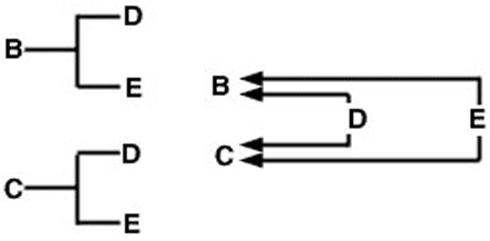
The use of this expression can be demonstrated with the full-sib sample pedigree and arrow diagram (Figure 1). In this example, assume neither sire nor dam is inbred. The arrow diagram on the right shows paths of gene flow from each of the common ancestors (D and E) to the animals whose coefficient of relationship we are measuring (B and C).
The problem now is to trace all possible paths from animal B to animal C that pass through a common ancestor. In this case, there are two such paths (Figure 2).
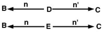
Since we have assumed no inbreeding in this example, the coefficient of relationship between animals B and C is estimated in Equation 3 below.
Equation 3
Usefulness of coefficient of relationship information
A livestock producer would find coefficient of relationship information valuable in a number of situations. He may, for example, want to sell an animal related to one that previously sold for a high price. The higher the coefficient of relationship between the two, the better its use as a sales point. Or he may want to purchase one of two related bulls and one may cost more than he wishes to pay. If the coefficient of relationship between the two bulls is high, he might be as well off with the lower priced bull as he would with the more expensive one.
A practical use of the coefficient of relationship is estimating the performance value of an untested animal. To estimate the value, we must know the performance value of a related animal, the coefficient of relationship between the tested and untested animals, and the average performance value of the breed, herd, or group to which the tested and untested animals belong.
As an example, consider a herd with a feedlot average daily gain (ADG) of 2.25 pounds per day. Assume further that a sire from this herd had a 3.50 pounds per day feedlot ADG, while a younger half brother has not, as yet, been evaluated for feedlot ADG. Assuming no inbreeding, the coefficient of relationship between half brothers is 0.25. The best estimate of the untested animal’s feedlot ADG is that it will deviate from the herd average 25 percent as far as does the performance value of the tested half brother. Using these figures, the most probable feedlot ADG value of the untested animal is 2.25 + (0.25) × (3.50 - 2.25) or 2.56 pounds per day.
Measurement of the degree of inbreeding
When we calculate an inbreeding coefficient, we are attempting to measure the probable percentage reduction in the frequency of pairing of dissimilar genes (reduction in heterozygosity). This reduction is relative to a base population. The base population usually is the breed concerned at a date to which the pedigrees are traced. Animals in this base population are assumed to be non-inbred. This does not mean these base population animals had dissimilar genes in each pair. There is no way for us to know how many of their gene pairs consisted of similar or dissimilar genes. The inbreeding coefficient that is calculated is simply relative to that base and reflects the probable percentage reduction in however many dissimilar gene pairs the average base population animals had.
The general expression for determining the inbreeding coefficient is estimated in Equation 4 below.
Equation 4
FX = S[(½)n + n' + 1 (1 + FA)]
where:
FX = the inbreeding coefficient of animal X.
S = Sigma, the Greek symbol meaning “add.”
(½) = the fraction of an individual’s genetic material that is transmitted to its progeny. It is used in the calculation of the coefficient of relationship because it represents the probability that, in any one generation, an identical gene from a given pair of genes is transmitted to each of two particular progeny. It is also the probability that an unlike gene from a given pair of genes is transmitted to the two progeny.
n = the number of generations between animal B and the common ancestor.
n' = the number of generations between animal C and the common ancestor.
+1 = is added to n and n' to account for the additional generation between animal × and its parents.
FA = the inbreeding coefficient of the common ancestor.
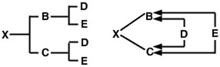
If neither parent is inbred, but if they are related, the inbreeding coefficient of their progeny is half their coefficient of relationship: ½ RBC This can be demonstrated using a full-sib mating to make comparison easy with the full-sib coefficient of relationship calculated previously. In this case, the pedigree for animal X and the arrow diagram will be as shown in Figure 3.
The problem now is to trace all possible paths from the sire (B) to the dam (C) through each common ancestor. As with the coefficient of relationship problem, there are two such paths:
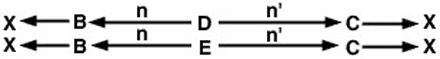
Since we have assumed neither parent is inbred, the inbreeding coefficient of animal × is estimated in Figure 5 as follows.
Equation 5
This is one-half the coefficient of relationship between full-sibs when there is no inbreeding.
Genetic consequences of inbreeding
The basic genetic consequence of inbreeding is to promote what is technically known as homozygosity. This means there is an increase in the frequency of pairing of similar genes. Accompanying this increase, there must be a decrease in the frequency of pairing of dissimilar genes. This is called a decrease in heterozygosity. These simultaneous events are the underlying reasons for the general effects on performance we observe with inbreeding.
Reasons for inbreeding
Development of highly productive inbred lines of domestic livestock is possible. To date, however, such attempts have met with little apparent success. Although occasional high performance animals are produced, inbreeding generally results in an overall reduction in performance. This reduction is manifested in many ways. The most obvious effects of inbreeding are poorer reproductive efficiency including higher mortality rates, lower growth rates and a higher frequency of hereditary abnormalities. This has been shown by numerous studies with cattle, horses, sheep, swine and laboratory animals.
The extent of this decrease in performance, in general, is in proportion to the degree of inbreeding. The greater the degree of inbreeding, the greater the reduction in performance. The actual performance reduction is not the same in all species or in all traits. Some characteristics (like meat quality) are hardly influenced by inbreeding; others (like reproductive efficiency) are greatly influenced by inbreeding. We cannot, then, make a generalized statement about the amount of reduction in “performance” that would result from a specific amount of inbreeding and expect it to be applicable in a broad variety of situations.
It is possible, however, to predict the extent of the effect of inbreeding on specific traits. Such predictions are based on results actually obtained under experimental conditions in which various levels of inbreeding had been attained. In research with swine conducted at the Midwest Regional Swine Breeding Laboratory, Dickerson and others (1954) point out that for each 10 percent increase in inbreeding (of the pigs in the litter), there is a decrease of 0.20, 0.35, 0.38, and 0.44 pigs per litter at birth, 21 days, 56 days, and 154 days, respectively. We can use such figures to provide estimates of expected decreases in litter size (at comparable litter ages) in other herds of swine.
Most inbreeding studies suggest each successive unit increase in inbreeding results in a proportional decrease in performance. Estimates of average increases in percentage inbreeding within a closed herd can be made with the expression:
(Number males + Number females) ÷
(8)(Number males)(Number females)
In a closed herd of cattle in which 100 females and four males were used in each generation, for example, the average per generation increase in inbreeding would be (4 + 100) ÷ (8)(4)(100) = 0.0325. On a per year basis, assuming a generation interval of five years, this would amount to an average yearly increase in inbreeding of 0.0065 or 0.65 percent.
Despite the generally poor results obtained with inbreeding, it is a very useful tool in animal breeding. Inbreeding is essential to the development of prepotent animals — animals that uniformly “stamp” their characteristics on their progeny. Because inbreeding causes an increase in the proportion of like genes (good or bad, recessive or dominant), the inbred animal’s reproductive cells will be more uniform in their genetic makeup. When this uniformity involves a relatively large number of dominant genes, the progeny of that individual will uniformly display the dominant characteristics of that parent.
Inbreeding may also be used to uncover genes that produce abnormalities or death — genes that, in outbred herds, are generally present in low frequencies. These harmful genes are almost always recessive in their genetic nature and their effects are hidden or masked by their dominant counterparts (alleles). Except for sex-linked traits, recessive genes are not expressed if carried singly. For their effects to be manifested, they must be present in duplicate. The likelihood they will be present in duplicate increases with inbreeding, because inbreeding increases the proportion of like genes (both good and bad) in the inbred population. With the effects of these genes uncovered, the breeder can eliminate them from his herd. He would cull progeny that showed the undesirable effect of these recessive genes and would also cull the parents that are carriers of the undesirable genes. In addition, two-thirds of the “normal” progeny of these carrier parents are themselves expected to be carriers of these same undesirable genes. In the absence of breeding tests to sort out the carriers from the non-carriers, it would also be necessary to cull all “normal” progeny of the carrier parents.
Breeders can use an inbreeding test to identify carriers of harmful autosomal recessive genes (like those responsible for snorter dwarfism in cattle, hyperostosis in swine, or cryptorchidism in sheep). An inbreeding test checks for only recessive genes that the tested animal (usually the male) carries. The following example and the numbers given are pertinent to cattle, where one offspring per gestation is usual. If we want to be sure at the 0.01 level of probability that a bull is free of harmful autosomal recessive genes, we would have to mate him to at least 35 of his daughters. He is mated to 35+ of his daughters because only half of them are expected to carry any harmful recessive gene their sire is carrying. We need the production of 35 normal calves without a single abnormal calf to show the bull free (at the 0.01 probability level) of any harmful autosomal recessive gene.
Tests in sheep and swine would require matings to fewer daughters. Actual numbers would depend on the average number of progeny produced per gestation in each species. Using the 0.01 probability level and assuming the average litter size is 1.5 in sheep and 8.0 in swine, the number of sire-daughter matings needed would be about 24+ for sheep and 5+ for swine.
Another important use of inbreeding is in the development of distinct families or inbred lines. Beginning with an initially diverse genetic population, inbreeding results in the formation of various lines, each differing genetically from the other. Continued inbreeding within these lines tends to change the frequency of some of the genes found in the initial population. For example, if a particular gene is present in only 1 percent of the animals in the initial population, inbreeding and the development of distinct lines could result in this gene being present in all or nearly all animals in some lines and in none or only a few of the animals in other lines. Inbred lines are used in a number of ways but are probably most notably used in the development of hybrid chickens or hybrid seed corn.
A generally mild form of inbreeding (linebreeding) is being used successfully by some seed stock and commercial producers. Its objective is to maintain a high degree of relationship between the animals in the herd and some outstanding ancestor or ancestors. With inbreeding in general, there is no attempt to increase the relationship between the offspring and any particular ancestor. In a linebreeding program there is a deliberate attempt to maintain or increase the relationship between the offspring and a specific admired ancestor (or ancestors). This feature distinguishes linebreeding as a special form of inbreeding.
The inbreeding coefficient of the offspring produced in a linebreeding program is generally low, but is dependent on the kind of breeding program followed. Figure 5 illustrates two linebreeding programs. The breeding program outlined in part A shows a direct line of relationship between offspring “x” and desired ancestor “5.” Only a mild level of inbreeding in animal “x” (Fx = 0.03125) is reached. The coefficient of relationship obtained between animal “x” and animal “5” is 0.2462. Part B is a linebreeding program based on continuous sire-daughter matings which, after only two generations, produces a level of inbreeding in animal “x” of 0.375 and a coefficient of relationship between animals “x” and “S” of 0.78.
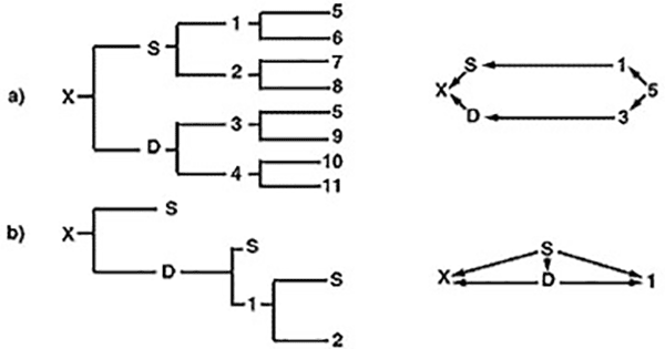
The sire-daughter program in part B effectively concentrates genes from animal “S,” but because of the rapid increase in inbreeding of the progeny produced in this program, the breeder runs the risk of greatly reduced performance and a high probability of genetic defects. Linebreeding programs are best used in purebred and high performing herds when a truly genetically superior individual in that herd has been identified and evaluated by progeny testing. Concentrating that individual’s genes would then be best accomplished by mating him to unrelated females to reduce the risk of harmful effects associated with such intense inbreeding.
Summary
Inbreeding is technically defined as the mating of animals more closely related than the average relationship within the breed or population concerned. For practical purposes, if two mated individuals have no common ancestor within the last five or six generations, their progeny would be considered outbreds. The primary genetic consequence of inbreeding is to increase the frequency of pairing of similar genes. All genetic and phenotypic changes associated with the practice of inbreeding stem from this one primary consequence. In general, inbreeding results in an overall lowering in performance. It is most obviously reflected in poorer reproductive efficiency, including higher mortality rates, lower growth rates and a higher frequency of hereditary defects. Despite these generally harmful effects, inbreeding is a very useful tool in the field of animal breeding. It enables the breeder to uncover and eliminate harmful recessive genes within the population. It is also essential to the development of prepotent animals and is desirable in the development of distinct family lines. In addition, seed stock and commercial producers have successfully used linebreeding to maintain a degree of genetic relationship in their animals to some outstanding ancestor or ancestors.
Glossary
The following terms describe various mating schemes and the progeny resulting from specific mating programs.
- backcross
Progeny resulting from the mating of a two-breed cross animal to one of the parental breeds. For example, using two breeds designated as P1, and P2, backcross progeny would be produced by mating the two-breed cross animal (Pl × P2) with either of the P1 or P2 parental breeds. - crisscrossing
A continuous program of crossbreeding in which there is an alternate use of males belonging to two breeds. Using two breeds designated as P1 and P2, a crisscrossing program, beginning with the two-breed cross animal (P1 × P2), would begin by backcrossing to one of the parental breeds [(P1 × P2) × P1]. Females resulting from these matings would be bred to a P2 male, [(P1 × P2) × P1] × P2, and so on. - crossbred
Progeny resulting from the mating of outcross animals belonging to different breeds. - genus cross
Mating of animals belonging to different genera (for example, mating of domestic cattle, Bos taurus or Bos indicus, to the American buffalo, Bison). - grading
Mating of purebred males of a given breed to non-purebred females and the resultant female offspring in successive generations. - inbred line
Line of animals produced by mating related animals. - inbreeding
Mating of animals more closely related to each other than the average relationship within the breed or population concerned. - incross
Progeny resulting from the mating of animals from different inbred lines within a breed. - incrossbred
Progeny resulting from the mating of animals from inbred lines of different breeds. - linebreeding
Generally mild form of inbreeding in which animals mated are related to some supposedly outstanding individual. - outbreeding
Mating of animals less closely related to each other than the average relationship within the breed or population concerned. - outcross
Progeny resulting from the mating of unrelated animals within a breed. - species cross
Mating of animals belonging to different species (for example mating of European breed cattle, Bos taurus, to Brahman cattle, Bos indicus). - three-breed rotational cross
A continuous program of crossbreeding in which males of three breeds are used on a rotational basis. Using three breeds designated as P1, P2 and P3, the first generation would involve production of two-breed cross animals, P1 x P2. In the second generation, two-breed cross females would be mated to males of the third breed, (P1 × P2) × P3; three-breed cross females would be mated to males of one of the breeds used to produce the two-breed cross animals, [(P1 × P2) × P3] × P1, and so on. - topcross
Progeny resulting from the mating of animals belonging to different families within a breed. - topcrossbred
Progeny resulting from the mating of inbred males to non-inbred females of another breed. - topincross
Progeny resulting from the mating of inbred males to non-inbred females of the same breed. - two-breed cross
Progeny resulting from the mating of males of one breed to females of another breed.
</p</p</p