Executive summary
- County government fiscal stress is defined as an increasing share of local income going to taxes.
- A long-term trend of population change may be a source of fiscal stress. To examine the relationship between population change and county fiscal stress, Missouri’s third class counties are classified into four population change categories: high-growth, medium-growth, slow-growth and population-loss.
- County costs are growing faster than costs in the economy as a whole.
- Population-loss counties are more likely to face fiscal stress due to increasing per capita costs as population falls.
- Slow-growth counties may face fiscal stress if costs rise faster than local income.
- Population-loss and slow-growth counties have increasing revenues per $100 of income. This is an indicator of fiscal stress. In addition, revenues per $100 of personal income are higher than in the other counties over the time period. This suggests that these counties may been in fiscal stress before 1996.
- Population-loss counties have higher per capita incomes than the other county types, but they still collect a higher share of income in taxes.
- High-population-growth counties may outgrow the existing capacity of some services and periodically make large investments to address capacity constraints. These periodic investments may leave high-growth counties temporarily exposed to fiscal stress. This exposure to fiscal stress decreases as the population continues to grow and the tax base increases.
- The medium-population-growth counties show the most stable tax revenues as a percentage of income.
- Another source of fiscal stress may be choices that counties make. Sales taxes are less stable than property taxes, but are the largest source of county revenues in all county types.
- Not all taxes are paid out of local personal income. Property taxes are paid by business and land owners who do not live in the county. Taxable sales may be made to businesses and consumers who do not live in the county. We do not have the data to estimate these outside contributions to local taxes.
Introduction
During the recent recession, local governments struggled to manage budgets as revenues dropped. Because the recession was deeper and longer than any in the past half-century, with a slower recovery, reserve funds were not sufficient.
With lower revenue, the majority of local governments struggled to meet the needs and expectations of citizens.
Since the Great Recession of 2008–2009, the budgets of local governments have not recovered at the same pace as the economy as a whole. The recession may have created greater demands for government services, and tax bases may have been affected by more cautious spending by businesses and consumers. Slow local budget recovery also may be due to state government decisions, such as changes in tax laws, stagnant or lower state aid, taxation constraints and increasing state mandated services (Aldag et al., 2017). An example of a state tax constraint is Missouri’s Hancock Amendment, which limits both state and local governments’ abilities to raise taxes. Elected local officials cannot raise taxes without voter approval (Kevin-Myers and Hembree, 2012). Finally, local governments’ decisions on taxes and tax incentives have major impacts on their own revenues (White, 2017).
Local budgets also are affected by longer-term trends, which, because they develop slowly, do not immediately come to the attention of local officials. For example, long-run changes to the economy affect tax bases, and the existing tax structures may not take these changes into account (White, 2017). The most common example is internet sales. A lesser-known fact is that American consumers are spending a larger share of their incomes on services, which generally are not taxed, and a smaller share on “things” that are subject to sales taxes. Another overlooked factor is that businesses pay sales taxes on some purchases, and business purchases have moved online to an even greater extent than have consumer purchases.
The long-run change in demographics is the focus of this analysis. Counties are experiencing changes in population size as well as in age groups. Population change, particularly rapid growth, often near cities and recreational areas, or population loss, often in agricultural counties, creates challenges for rural local governments as it affects governments’ tax bases and the number of people who must be provided government services. Outmigration reduces the number of young adults in the labor force, and many rural counties have a predominantly elderly population.
As population changes, counties’ per capita costs of providing services change in two ways. First, economies of scale exist when an increase in production results in a decrease in the per unit cost of production. A similar idea for counties is the per unit cost of a service, which can be thought of as the cost per citizen or per capita cost. Counties with growing populations may find that the per capita cost for a service decreases as they increase the total amount of the service to provide it to more citizens. However, counties with small populations have limited ability to lower per capita costs. If they lose population and produce a lower total amount of a service, the per capita cost of providing that service increases. Second, for some services, such as roads, counties may need to continue to produce the same level of services, but if that cost is spread among fewer people, the per capita cost per mile increases.
If population is growing, the county may be able to provide services to more people at a lower cost per person. At the same time, rapid population growth may create capacity constraints that require large investments to accommodate the growing population. For example, there may be increasing congestion on a bridge, creating a need for additional lanes. Generally, when such improvements are made, additional capacity is constructed to accommodate future growth. The initial investment may increase the per capita cost of services even though the population is growing. However, once the initial investment is made, the per capita bond repayment and operational costs decrease as population grows.
Maher and Nollenberger (2009, p. 62) define “financial condition” as “an organization’s ability to maintain existing service levels, withstand economic disruption, and meet the demands of growth and decline.” In this case, we expect that counties with declining populations or very slow growth may face the difficulty described above, even in the absence of a recession. Fiscal stress may be thought of as a county’s increasing difficulty or inability to meet these criteria. Because all taxes are paid out of income, for this analysis, fiscal stress is defined as an increasing share of local income being paid in taxes. This is measured as tax receipts per $100 of local income, or as a percentage of income.
Population
To examine the relationship between county population change and county fiscal stress, Missouri’s third class counties are divided into four groups based on population change from 1996 to 2017, a 22-year period. High-population growth counties grew faster than the state average from 1996 to 2017, medium-growth counties grew at a rate between the state average and the average of third class counties, and slow-growth counties grew slower than the average third class county. Population-loss counties lost population over this period. Webster, Pulaski and Warren counties, three counties classified as very high growth counties (having grown 37.7%, 38.4%, and 55.2% respectively), are excluded from this analysis because their growth rates are not comparable to other counties and because of the inability to make meaningful generalizations from just three counties.
The map (Figure 1) shows how each third class county is classified by population change. Most high- and medium-growth counties are clustered around growing urban areas, many of them the smaller urban areas in the state, and in recreation and tourism regions, such as the Lake of the Ozarks, Branson and the nearby lakes. A unique cluster of fast growth is around Pulaski County (itself a third class county that grew 38%) where Fort Leonard Wood is located. Most counties north of the Interstate 70 corridor lost population or grew more slowly than the average third class county. There is also a cluster of population loss counties in the Bootheel in southeastern Missouri. A majority of population-loss counties are agricultural or resource-dependent counties, such as Iron and Reynolds in the southeast, which are historically dependent on mining (ERS, 2017).
The county population groups are compared to see if population change is associated with fiscal stress. If per capita income is similar across county types, it is expected that population-loss counties’ tax revenues will be a higher percentage of income than in the other counties, that is, they are more likely to be experiencing fiscal stress. High-growth counties may also experience fiscal stress if they reach capacity constraints.
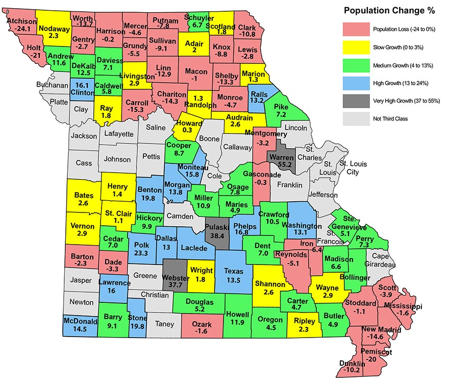
Figure 1. Third class counties by population change: 1996–2017 (see Table 1 below).
Table 1. Third Class County Population Growth Rates (1996–2017).
| Population-loss counties | |
|---|---|
| Name | Population change |
| Atchison | -24.12% |
| Barton | -2.32% |
| Carroll | -15.27% |
| Chariton | -14.31% |
| Clark | -10.81% |
| Dade | -3.28% |
| Dunklin | -10.22% |
| Gasconade | -0.26% |
| Gentry | -2.74% |
| Grundy | -5.52% |
| Harrison | -0.19% |
| Holt | -20.98% |
| Iron | -6.36% |
| Knox | -8.81% |
| Lewis | -2.77% |
| Linn | -12.94% |
| Macon | -1.03% |
| Mercer | -4.57% |
| Mississippi | -1.59% |
| Monroe | -4.72% |
| Montgomery | -3.16% |
| New Madrid | -14.55% |
| Ozark | -1.58% |
| Pemiscot | -20.04% |
| Slow-growth counties | |
|---|---|
| Name | Population change |
| Adair | 1.99% |
| Audrain | 2.59% |
| Bates | 2.56% |
| Henry | 1.43% |
| Howard | 0.32% |
| Livingston | 2.92% |
| Marion | 1.33% |
| Nodaway | 2.26% |
| Randolph | 1.28% |
| Ray | 1.79% |
| Ripley | 2.25% |
| Saint Clair | 1.12% |
| Scotland | 1.83% |
| Shannon | 2.57% |
| Vernon | 2.93% |
| Wayne | 2.90% |
| Wright | 1.77% |
| Medium-growth counties | |
|---|---|
| Name | Population change |
| Andrew | 11.62% |
| Barry | 9.09% |
| Bollinger | 7.76% |
| Butler | 4.92% |
| Caldwell | 5.83% |
| Carter | 4.65% |
| Cedar | 7.00% |
| Cooper | 8.73% |
| Crawford | 10.48% |
| Davies | 7.11% |
| DeKalb | 12.49% |
| Dent | 6.99% |
| Douglas | 5.21% |
| Hickory | 9.89% |
| Howell | 11.92% |
| Madison | 6.60% |
| Maries | 4.92% |
| Miller | 10.92% |
| Oregon | 4.51% |
| Osage | 7.84% |
| Perry | 7.34% |
| Pike | 7.18% |
| Sainte Genevieve | 5.12% |
| Schuyler | 6.65% |
| High-growth counties | |
|---|---|
| Name | Population change |
| Benton | 19.84% |
| Clinton | 16.07% |
| Dallas | 12.97% |
| Laclede | 16.88% |
| Lawrence | 16.01% |
| McDonald | 14.47% |
| Moniteau | 15.78% |
| Morgan | 13.83% |
| Phelps | 16.75% |
| Polk | 23.33% |
| Ralls | 13.22% |
| Stone | 19.83% |
| Texas | 13.53% |
| Washington | 13.12% |
| Very high-growth counties | |
|---|---|
| Name | Population change |
| Pulaski | 38.39% |
| Warren | 55.15% |
| Webster | 37.71% |
Tax base trends
Tax bases are the resources available to governments to raise revenue. The two major tax bases for Missouri counties are assessed property values and taxable sales. Businesses contribute to the property tax base because they own property. Businesses contribute to the sales tax base by making taxable sales to their clientele as well as making some purchases that are taxable. Counties also raise revenues from fees and charges, which are most often dedicated to a specific purpose.
Although Missouri counties do not directly tax income, all taxes are paid from income. Thus, income is the indirect tax base for the counties. For a county to provide a given level of services, the higher the total income of a county’s residents, the lower the average tax rate necessary. Difficulty meeting budgets is one reason why some counties might be collecting more revenue relative to resident income, defined as fiscal stress.
But there are positive reasons why some counties may be collecting more revenue relative to residents’ incomes: 1) there are more businesses in the county than in most others or 2) more tax revenue comes from non-residents than in other counties (sales taxes or property owners who do not live in the county). However, there are no data on taxes paid by non-residents nor are data readily available on local taxes paid by businesses. 3) Finally, it might also suggest that citizens of the county want higher levels of services and are willing to pay for them.
Per capita income and inflation
Because all taxes are paid from income, the measure of fiscal stress is an increasing share of local income being paid in taxes. The average income of county residents (per capita income) is a general indication, as noted above, of income available in the county to pay for services. Inflation decreases the purchasing power of a given income. To account for the increasing costs for goods and services, personal income is adjusted for inflation, using the Consumer Price Index (CPI).
Figure 2 compares both nominal and real per capita income by county population groups.
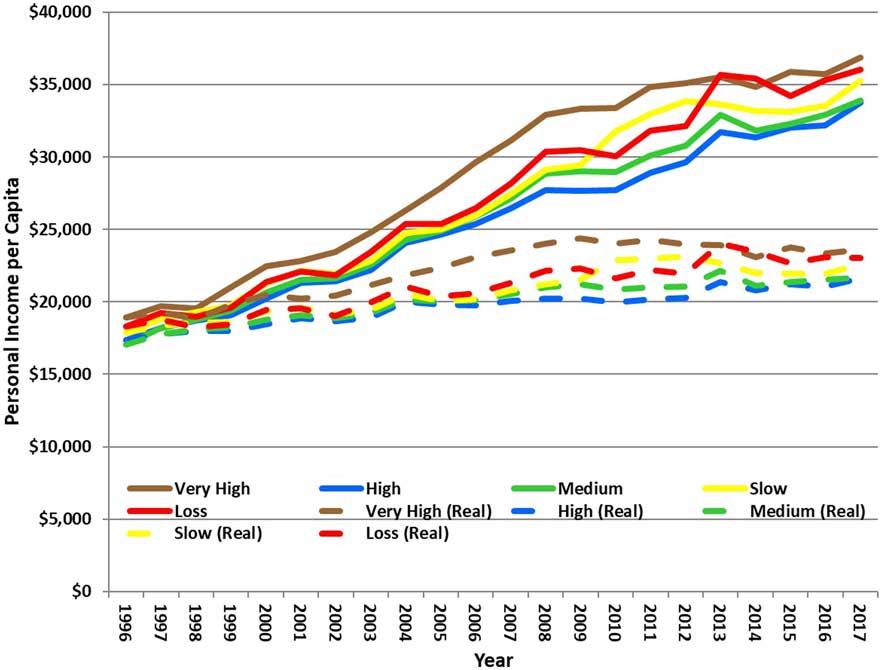
Figure 2. Per capita income by population change, nominal and real.
The high-population growth counties generally have the lowest per capita income. Population-loss counties generally have the highest per capita income over the period. The per capita income of slow-growth counties is similar to that in population-loss counties. The population-loss and slow growth-counties tend to be agricultural, and the agricultural economy was strong through much of the period before its growth slowed towards the end of the period.
The upper and lower sets of lines on the graph compare nominal (or current) per capita income and real (adjusted for inflation) per capita income for each population group. The graph shows that while nominal per capita income nearly doubled from 1996 to 2017, real per capita income increased between $4,250 in high-growth counties and $4,730 in population-loss counties. While less than the increase in nominal income, it does indicate that this indirect tax base is growing per capita in purchasing power.
Inflation not only decreases the purchasing power of residents’ income, it also decreases the purchasing power of government revenues. Government costs include things that households do not buy, such as asphalt or election software, and governments tend to purchase wholesale, while consumers purchase retail. The Municipal Cost Index (MCI) shows the effects of inflation on the costs of providing local government services, and the CPI shows the effects of inflation on the costs of consumer goods and services (Penton Media, 2018).
Figure 3 compares the MCI with the CPI in 1996 dollars. After 2004, the MCI increased faster than the CPI, indicating that municipal service costs increased faster than the costs of consumer goods and services. A given revenue for the county will purchase less, and a county may have to raise taxes. Whether this will result in a higher share of citizens’ income going to taxes (the indicator of fiscal stress) will depend on how fast consumers’ income is growing.
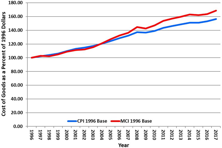
Figure 3. MCI and CPI from 1996 to 2017.
Per capita costs
A county’s total expenditures from the general fund are its total costs for this analysis. Expenditures from special funds, for example, the road and bridge fund and special sales tax funds, are not included. Figure 4 shows both nominal and real (adjusted for inflation) total expenditures. While all county types show an increase in nominal total expenditures over the period, the use of real dollars shows a different story. All counties had an increase in real total expenditures in the late 1990s and early 2000s, but trends began to diverge around 2004. Real per capita expenditures in medium- and high-growth counties decreased for some years before rising again. There is more volatility in per capita expenditures in high-growth than medium-growth counties.
Population-loss and slow-growth counties had the greatest increase in per capita expenditures with real expenditures ending the period $44.66 and $32.36 per capita higher than they started. This fits with the expectation that counties face higher costs as they lose population. For the slow-population-growth counties there was little increase in real per capita expenditures until about 2014 when real per capita costs increased. This suggests that costs are rising faster than population in slow-growth counties.
The high-growth counties’ real expenditures per capita increased by $10.15 over the period, and medium-growth counties’ real expenditures increased by $2.53 per capita. The higher increase in per capita costs for high-growth compared with medium-growth counties may be a result of large infrastructure investments or increasing costs of other services that may be required to meet needs in high-growth counties.
It is expected that the increasing per capita costs may cause fiscal stress for counties. Fiscal stress is defined as an increasing percentage of personal income in the county going to taxes and fees.
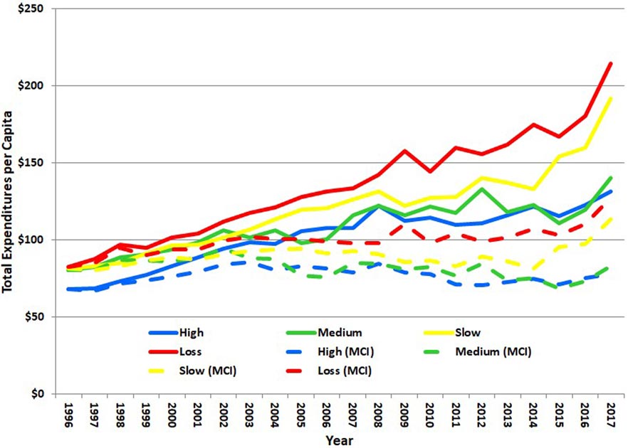
Figure 4. Total expenditures per capita by population change.
Tax bases
Counties have two major tax bases — assessed property value and taxable sales. Assessed property value includes real estate, livestock, grain, agricultural and pollution control equipment, and personal property. By far the largest is real estate. Assessed property values are generally less volatile than taxable sales (Stallmann and Johnson, 2011). The assessed value of real estate changes slowly because it is a long-run investment whereas taxable sales tend to be based on short-run decisions and are more responsive to changes in the economy. Reliance on unstable tax bases may create fluctuations in county revenue and fiscal stress.
Tax bases per capita
Figures 5 and 6 show the difference in stability between assessed property value per capita and taxable sales per capita. To show the real purchasing power of the tax bases, the lower part of the two graphs shows the two tax bases adjusted for inflation by the MCI. Before the financial and housing bubble in 2007, real taxable sales per capita increased in all counties. During and after the subsequent recession, real taxable sales per capita decreased in all counties. In all but the medium-growth counties real taxable sales per capita have not recovered to the levels of 1996. In the medium-growth counties real taxable sales are $30 per capita higher in 2017 than in 1996. However, during the same period, assessed property values are more stable. In all of the county types real assessed values per capita declined during the recession but did not fall below 1996 values. By 2017, assessed values per capita are $1,000 higher than 1996 in the slow-growth counties, $1,500 higher in the population-loss and high-growth counties, and $1,800 higher in the medium-growth counties.
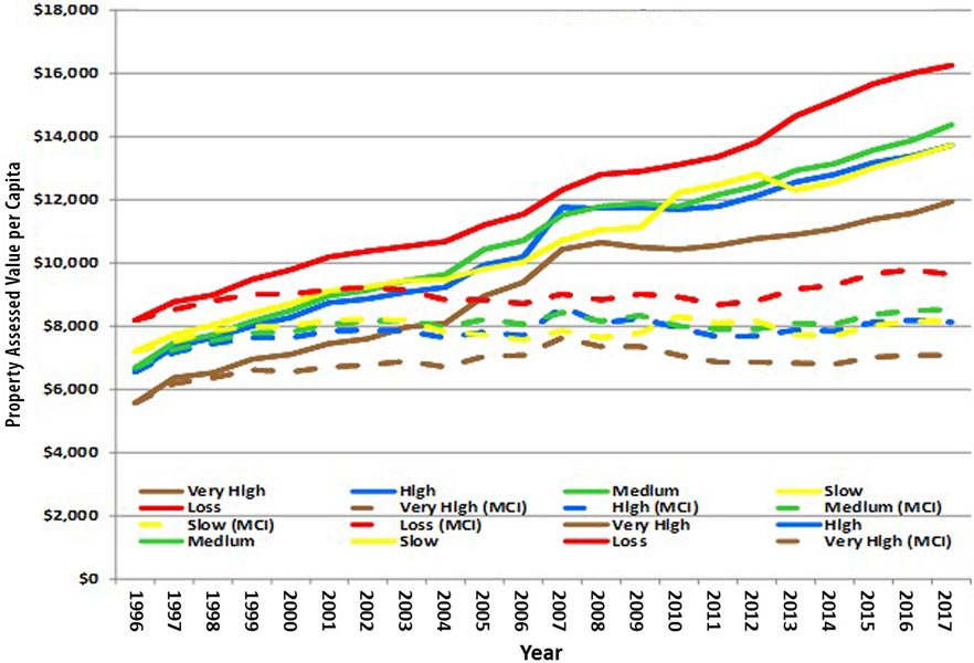
Figure 5. Property assessed value per capita by county population change, both nominal and MCI adjusted.
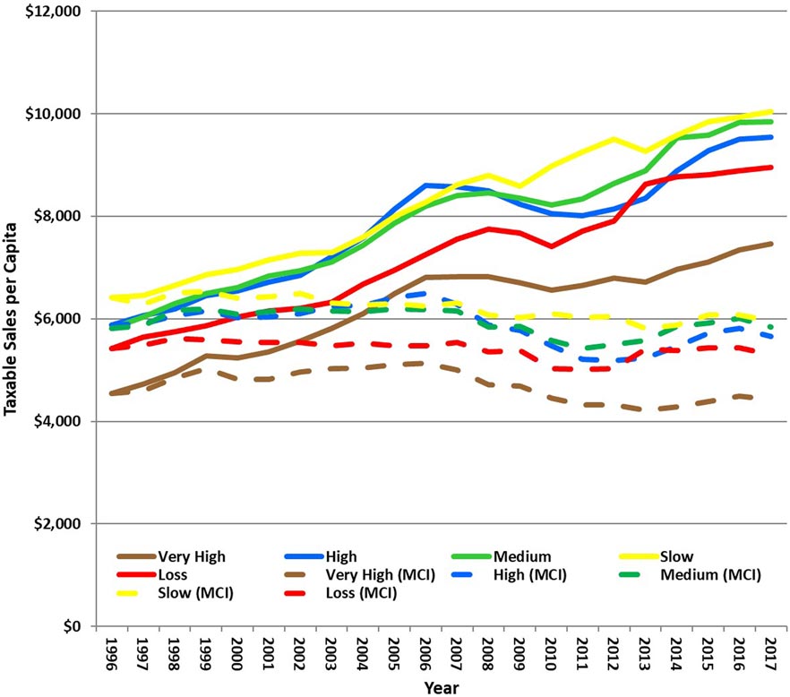
Figure 6. Taxable sales per capita by county population change, both nominal and MCI adjusted.
There are two primary reasons why population-loss counties have the highest assessed property value per capita. First, these counties are agricultural. Agricultural land is assessed at use value, which does not grow rapidly, but did not decline because the agricultural economy was strong through most of the period. Second, population loss means that the total assessed value is divided by a smaller number of people, increasing assessed values per capita.
While people who live outside of the county likely own some of the land and pay the taxes, the per capita measure is a measure of the tax base available per capita for the county to use.
Taxable sales consist of both retail sales and purchases made by businesses. Population-loss counties have the lowest taxable sales per capita. Counties losing population or with a slow-growing population are not likely to have large businesses making taxable purchases. These counties likely have small retail sectors because there is not sufficient demand to make a variety of outlets profitable. In addition, if there are few jobs, people may commute out of county to work. Commuters likely earn higher incomes than if they did not commute. This increases the income they could spend locally, but they also have opportunities to make purchases where they work. Commuters are likely to spend more of their income outside of their home county than do non-commuters with the same income.
The value of assessed property and taxable sales, coupled with the decision of which tax base to rely on more heavily, affects the county’s ability to generate revenue. Population-loss counties have higher assessed property values per capita than the other county types, but they also have the lowest taxable sales per capita. While assessed property value per capita is higher than taxable sales in all counties, the gap between the two is largest in population-loss counties. This suggests that a heavy reliance on sales taxes by population-loss counties will require a high sales tax rate, which could discourage shoppers and businesses.
Tax bases per $100s of income
Comparing assessed property values per $100s of income with taxable sales per $100s of income further illustrates the differences in the stability of the two tax bases. Figures 7 and 8 show that both per capita income and per capita assessed values per $100 of income increased. Assessed property values per $100s of income (Figure 7) in all county groups show stability over time. (Because the comparison per $100 of income is a ratio, either the nominal or real values will provide the same ratio.) Assessed values per $100 of income increased by $3 over the period in high- and medium-growth counties. Assessed property values per $100 of income in population-loss were the same at the beginning and end of the period. Slow-growth counties decreased $1 by the end of the period. A decrease suggests that, in general, incomes grew more rapidly than property values. As noted above, agricultural land is assessed at use value and grows slowly. With a strong agricultural economy during much of the period, it is likely that incomes grew more rapidly than assessed values.
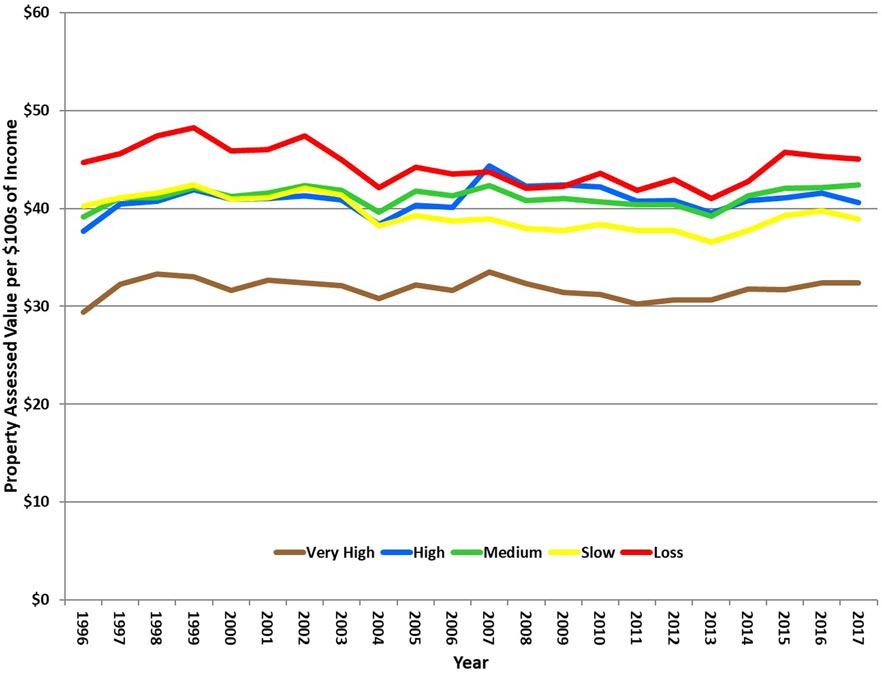
Figure 7. Property assessed value per one hundred dollars of income by county population change.
On the other hand, Figure 8 shows taxable sales per $100 of income have a downward trend in all county types. Taxable sales per $100 of income continued to fall even after the recovery from the recession began and have not recovered to pre-recession levels. Because per capita income increased during the period, this shows that income grew more rapidly than taxable sales. There may be a number of explanations for this, such as increased consumer frugality in the wake of the recession, increased internet sales to both consumers and businesses, some of which is not taxed, and increased spending on services, most of which are not taxed in Missouri.
Comparing the two graphs shows that assessed property values are a more stable tax base than taxable sales. Property is a long-run investment, while taxable sales are responsive both to short-run economic changes, such as the recession, and to longer-run, changing consumer purchasing patterns.
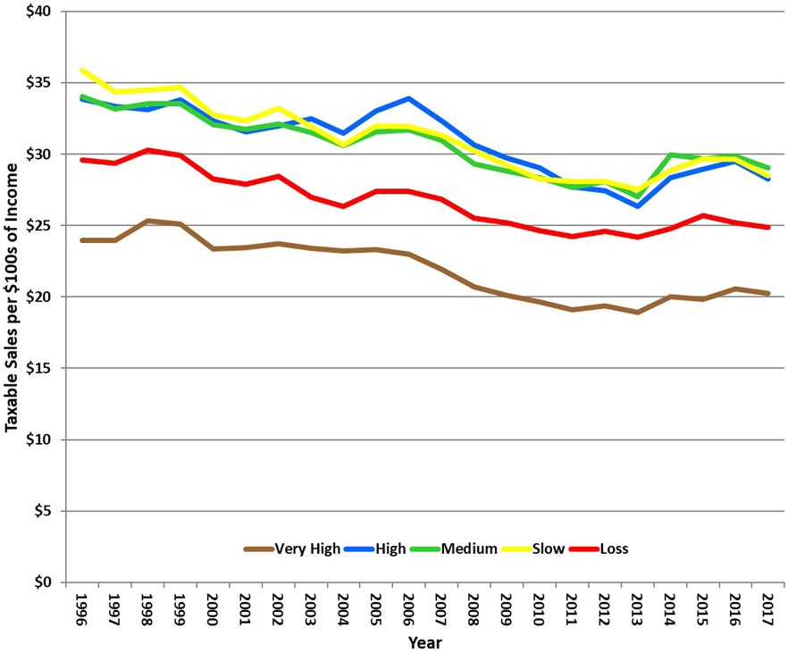
Figure 8. Taxable sales per one hundred dollars of income by county population change.
Tax bases and fiscal stress
The size and stability of the county’s tax bases, citizens’ income, and the relative costs of providing public services are all factors affecting county fiscal decisions. Tax base size and stability are important to how resilient a county may be to changes in the economy. Higher reliance on more stable tax bases offers more resilience than a reliance on unstable tax bases. Another important consideration is how much of their income residents are paying in county taxes. If residents are paying a relatively high or increasing proportion of their income in county taxes, this is an indicator of fiscal stress.
Counties with higher per capita income may be less likely to experience fiscal stress. Finally, inflation has increased the costs of goods and services purchased by local governments faster than the costs of general consumer goods (Figure 3). This may cause counties to raise taxes. Whether this will result in taxes becoming an increasing percentage of income will depend on if income is growing slower or faster than county costs.
County revenues
County governments draw revenue from their major tax bases, indirectly from residents’ incomes, from fees and charges, and from higher levels of government or as part of agreements with other counties. Revenues from fees and charges and other governments may be restricted in their use.
An increasing proportion of citizen income going to pay county revenues is an indicator of potential fiscal stress. Alternatively, the county might be receiving revenue from non-residents whose income is not included in the county data. For example, property owners who live outside the county pay taxes as do non-residents who shop in the county. Information on non-residents paying taxes is not available. Finally, it might also suggest that citizens of the county want higher levels of services and are willing to pay for them. To determine if the latter is the case would require polling citizens about their demand for public services.
Information about county budgets
The data for county revenues are from the annual budgets that third class counties submit to the state. Annual county budget documents contain three years of data: actual data for the past year, data for the current year, which is a mix of actual data and projections for the rest of the year, and the projected budget for the next year. The most recent data are from the budget document for 2017, which means 2017 is a projection and the data for 2016 are not the final numbers for the 2016 year. From 2005 onward, the data are not audited and may contain errors. It is unlikely that an error in a single county will have a large impact on the average for a group of counties.
In examining the fiscal trends in the following graphs, it is important to remember that the data for 2016 and 2017 are not the final budget numbers for those years and 2015 is the most recent actual data. In addition, counties report their budgets in several formats so that we do not have data on every third class county for every year. For each year, we calculate the trends in the fiscal ratios using only the counties for which there are standard budgets for that year.
The ratios presented below do not include debt. As a result, the ratios focus on short-term budget trends and how they compare across county population growth types.
Total receipts
Total receipts for a county include property taxes, sales taxes, and fees and charges, all of which are paid out of income. The other major part of receipts is intergovernmental revenues, which can be thought of as an addition to county income. The discussion of total receipts includes all of these sources, followed by an examination of each source.
Figure 9 shows that total receipts per $100 of income increased from 1996 to 2017 by $0.04 and $0.05 per $100 of income in slow-growth and population-loss counties respectively. High population-growth counties’ receipts per $100s of income increased $0.05 from 1996 to 2006. Since then, receipts per $100s of income in high-growth counties have decreased to $0.02 below their 1996 level. For medium-growth counties the decline is more pronounced — total receipts decreased $0.10 per $100 of income. Even though population-loss counties have higher per capita income, the increase in receipts per $100 of income suggests the higher per capita income is not sufficient to avoid fiscal stress. It also is worth considering that the residents may be willing to pay higher taxes because of other factors they find valuable, such as quality of life, open space, small communities, etc.
To put these changes per $100s of income into perspective, if a county resident makes $50,000 per year, and the county receives $0.05 per $100s of income more at the end of the period than at the beginning, that means the resident pays $25 more in taxes in 2017 than in 1996. If the change is $0.10 per $100 of income, the resident pays $50 more in taxes.
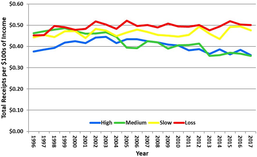
Figure 9. Total receipts per one hundred dollars of income by population change.
Property and sales tax receipts
Counties adjust to various economic and fiscal conditions by changing their reliance on property taxes, sales taxes, and fees and charges for services. While the proportion of revenue collected to the amount of income in the county is an indicator of the county’s current fiscal condition, relative reliance on one revenue source over another may make a county fiscally susceptible to changes in the economy or to policy decisions made at higher levels of government. In addition to economic conditions, preferences of citizens affect a county’s decision to rely on different sources of revenue.
Property and sales taxes are paid by anyone who owns property in the county or purchases taxable goods in the county, whether they are residents or not. Counties that receive a lot of revenue in property and sales taxes from non-residents may be better off fiscally because they are receiving revenue from people who do not require as many government services as residents. This potential benefit would be reflected by higher tax revenues per $100s of income (Figures 10 and 11) because non-resident income is not included in the measure while taxes paid by non-residents are. We are not aware of sources for data on taxes paid by non-residents.
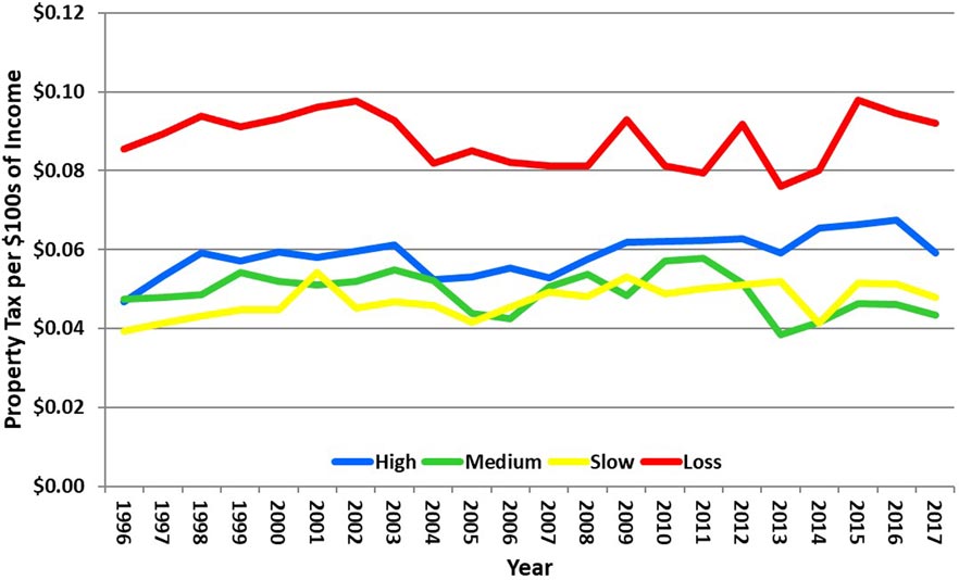
Figure 10. Property tax revenue per one hundred dollars of income by population change.
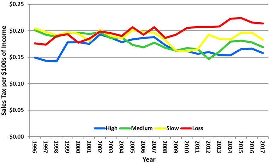
Figure 11. Sales tax revenues per one hundred dollars of income by population change.
Population-loss counties generally received between $0.08 and $0.10 per $100s of income in property taxes over the time period, approximately twice what the slow- and medium-population-growth counties received during the same period. The high-growth counties show a slight upward trend during the period. Early in the period their rates fluctuated between $0.05 and $0.06 and ended the period above $0.06. Population-loss counties’ greater reliance on the property tax, compared to the other counties, may be a response to relatively low taxable sales, as shown in the taxable sales per $100 of income graph (Figure 8).
From 2008 to 2017, of the four county types, population-loss counties had the highest sales tax revenue per $100 of income, and the trend is increasing. These counties have both the lowest taxable sales per capita and the lowest taxable sales per $100 of income, as well as a declining trend in taxable sales per $100 of income. The increase in revenues suggests that sales tax rates have been raised and are higher than in the other counties.
All of the counties have declining taxable sales per $100 of income, yet the loss-, slow- and high-population counties do not have a declining sales tax revenue trend. This means that the counties have raised tax rates. Only the medium-income counties have a revenue trend with an overall small decline.
Figures 10 and 11 show that, in general, population-loss counties are exerting a greater tax effort than are other county types. This suggests either that citizens of these counties are willing to pay more for county services or that population-loss counties are experiencing more fiscal stress than other county types. Current fiscal stress may leave them more vulnerable to future economic changes. If an economic downturn leads to a decrease in taxable sales, it may be more difficult for population-loss counties to increase property taxes to make up for their losses than it would be for other county types, because population-loss counties already have higher property taxes per $100s of income.
Across all county types, sales tax revenues are a higher percentage of income than are property tax revenues. All county types receive between $0.15 and $0.22 per $100s of income in sales taxes and between $0.04 and $0.10 per $100 of income in property taxes. As the taxable sales per $100s of income graph shows, taxable sales are more responsive to changes in the economy than are assessed property values. Thus taxable sales may lead to uncertainty in county fiscal planning. In some county types, non-residents are contributing to sales tax revenues
Fees and charges for services
Fees and charges for services are another source of revenue for county governments that are large enough to affect a county’s fiscal condition and stability. Fees and charges for services are paid to engage in certain activities, such as obtaining a business license, or receiving a specific service from the county, such as filing the title on a piece of property. Figure 12 shows that the percentage of income paid for fees and charges for services is comparable to what is paid in property taxes in most county types (Figure 10).
The exception is slow-growth counties, where fees and charges are twice that of property taxes per $100 of income. From 1996 to 2017, fees and charges as a share of income increased in the slow-growth counties from about $0.09 to between $0.13 and $0.14 per $100s of income near the end of the period. Slow-growth counties may be using fees rather than property taxes, which are relatively low in comparison with the other counties. It may be that citizens prefer fees and charges to property taxes.
Fees and charges for services per $100s of income decreased in high- and medium-population-growth counties. In population-loss counties, fees and charges for services per $100 of income fluctuated over the time, first showing a downward trend, but rising with the recession to just over what they were in 1996. At the end of the period, population-loss counties have the second highest fees and charges per $100 of income and the highest property and sales tax per $100s of income of all counties. This suggests that these counties likely are experiencing fiscal stress.
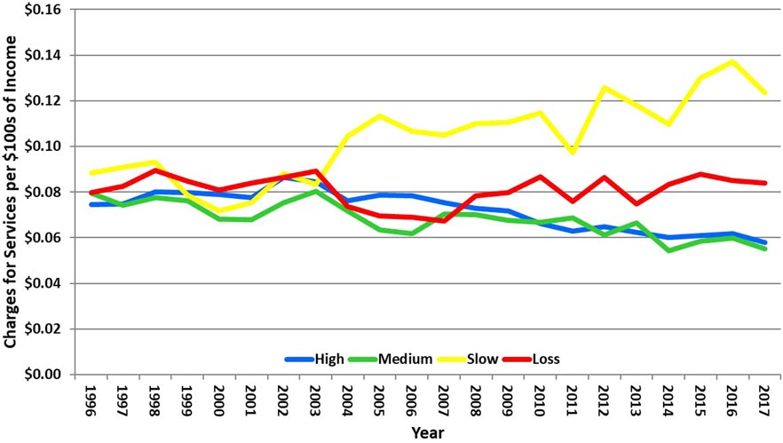
Figure 12. Fees and charges for services per one hundred dollars of income by population change.
Intergovernmental funds
In general, intergovernmental funds can be thought of as an addition to county revenues rather than a tax that is paid to the county. Thus intergovernmental revenues per $100 of income is how much additional revenue is coming into the county as a percentage of county income. One exception to this is revenue from the financial institutions tax. The state, not local governments, sets the rate (currently 7% of net income) and collects the tax. The state retains a collection fee, and the revenues are sent to the county in which the institution is located (Department of Revenue, 2017).
Intergovernmental funds are from higher levels of government and also from contracts between various local governments. Of these sources, only contracts with other local governments are under the direct control of the county. All other intergovernmental revenues are due to decisions made at higher levels of government — which programs to support and how much funding to allocate for them. These funds vary in purpose and may be one-time grants or long-term financial commitments. It should be noted that special purpose funds, such as for roads and bridges, are not part of the general fund. The extent to which counties can control how much revenue they receive from higher levels of government is limited to their ability to apply for grants and to control whatever characteristics within the county the programs target (public health, safety, infrastructure, etc.). This means that intergovernmental funds can be volatile and may not be readily available during periods of fiscal restraint by higher levels of government.
Figure 13 demonstrates the volatility of intergovernmental funds. High-growth counties have the most stable intergovernmental receipts throughout the period, but with a declining trend. For all other county types, intergovernmental receipts show volatility throughout the period. Medium-growth counties show both volatility and a declining trend. Slow-growth and population-loss counties show the most volatility and end the period at about the same intergovernmental revenues per $100 of income as at the beginning of the period. The volatility of these funds makes management and planning more difficult and likely contributes to fiscal stress.
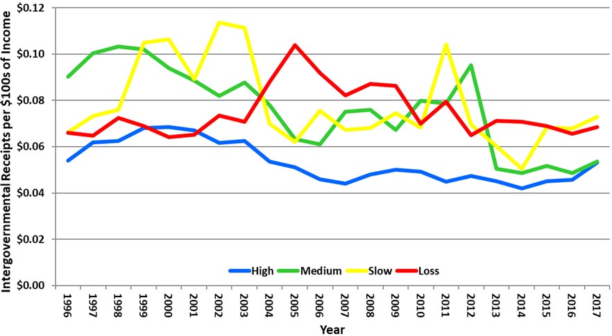
Figure 13. Intergovernmental receipts per one hundred dollars of income by population change.
Cash balances
General revenue funds are receipts from property taxes, sales taxes, intergovernmental funds, fees and charges for services, interest, and other miscellaneous receipts that do not come from a dedicated tax or are not received for a dedicated purpose. The Government Finance Officers Association recommends that governments end the fiscal year with sufficient funds to cover no less than the first two months of the next fiscal year (Gauthier, 2009). Cash balances also help the county manage fluctuations in revenue and expenditures that are not planned. Gauthier recommends that smaller governments maintain a larger general fund balance as a percentage of annual expenditures because it can be particularly difficult for small governments to accommodate unforeseen expenditures. For example, a single unexpected expenditure, such as a large court case, will take a larger percentage of a small government’s budget than of a larger government’s. Gauthier finds that many local governments maintain fund balances insufficient to prevent fiscal stress in the event of a fiscal shock.
The cash balances of the slow-growth counties show the most volatility (Figure 14). The population-loss and slow-growth counties increased their cash balance per $100s of income during the Great Recession and continued to do so until the last few years. This may have been a conscious decision to be more frugal during a time of economic hardship and to avoid greater fiscal stress in the near future. The cash balances of the high-growth counties remained relatively steady over time. The cash balances of the medium-growth counties show some volatility and an overall downward trend.
While all of the county groups show a projected drop in cash balances in 2017, this may be because this is a projection and not a number from a completed budget year.
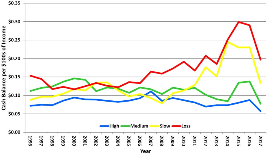
Figure 14. Cash balance per one hundred dollars of income by population change.
Summary
For the analysis of the fiscal position of third class counties, the indicator of fiscal stress was defined as an increasing share of local income going to taxes. Population change affects Missouri counties’ resilience to fiscal stress. Population loss increases per capita costs, requiring a greater tax effort to maintain services. Differing economic factors between counties may alleviate or magnify the effects of population loss. For example, population-loss counties in the agricultural area in northern Missouri may have benefited from a strong agricultural economy during much of the period examined, while non-agricultural population-loss counties in southern Missouri may have experienced greater fiscal stress. High-population-growth counties must periodically address capacity constraints, which may result in periodic fiscal stress that can be exacerbated by economic shifts. An understanding of how population change affects county fiscal condition can help county governments adopt policies to make county finances more resilient to fiscal stress.
The total receipts per $100s of income graph (Figure 13) indicates that from 1996 to 2017 population-loss and slow-population-growth counties increased total receipts per $100 of income, an indicator of fiscal stress. With higher per capita costs to begin with and population loss contributing to increasing per capita costs, population-loss counties collected more revenue per $100s of income in property and sales taxes than any other county type. In comparison with other counties, population-loss counties have relatively higher per capita incomes during most of the period. Yet the higher income did not alleviate fiscal stress, as these counties collected more revenue per $100 of income than did other counties. Population-loss counties may struggle to adapt to economic and fiscal changes more than other counties because their tax effort is already greater than other counties.
High-growth counties experienced increasing receipts per $100 of income early in this period, perhaps due to hitting capacity constraints, which needed to be addressed. The large investments required to increase the capacity of infrastructure to accommodate a growing population can cause periodic fiscal stress while the investment is made. The timing of necessary infrastructure investments may leave high-growth counties vulnerable if the investments coincide with an economic downturn. From the mid-2000s onward, receipts per $100 of income show a declining trend in high-population-growth counties, suggesting that counties in this group are less likely to be experiencing fiscal stress now.
The medium-growth counties have a declining trend of receipts per $100 of income, suggesting that counties in this category are the least likely to have experienced fiscal stress during the period.
This analysis explored how population change might affect fiscal stress. But other factors are also at work that are specific to each county. For example, the economic structure of the county might be more or less resilient to economic changes. Tourism counties, for example, are more likely to face fiscal stress because tourism responds rapidly in an economic downturn. In addition, counties have limited ability to affect the intergovernmental revenues they receive.
Choices that counties make also may affect fiscal stress. The tax base that counties rely on can affect their fiscal stress. Reliance on sales taxes, which are more responsive to short-run economic shifts than other tax bases, may increase revenues during good economic times, but result in revenue shortfalls in an economic downturn. For all county types, sales taxes are a higher share of income than are property taxes, which are a more stable tax base. The population-loss counties collect a higher share of income in both sales and property taxes than the other county types, suggesting they may be more vulnerable to fiscal stress in the future. Slow-growth counties rely more on fees and charges than on the property tax, but fees and charges are more volatile than the property tax. In addition, many counties have special funds for law enforcement, jail, economic development, etc., often funded by sales taxes. This increases the counties’ exposure to fiscal stress in an economic downturn.
References
- Aldag, Austin M. and Mildred E. Warner, and Yunji Kim. (2017). “What Causes Local Fiscal Stress? What Can Be Done About It?” Department of City and Regional Planning, Cornell University Ithaca, NY.
- Bel, Germá and Mildred E. Warner. (2015 ). “Inter-Municipal Cooperation and Costs: Expectations and Evidence.” Public Administration. 93(1March): 52-67.
- Brown, K.W. (1993). “The 10-Point Test of Financial Condition: Toward an Easy-to-Use Assessment Tool for Smaller Cities.” Government Finance Review. 9(6, December): 21-26.
- Department of Revenue. (2017). “Local Government Tax Guide.”
- Economic Research Service (ERS). (2017). “County Economic Types, 2015 Edition.” United States Department of Agriculture.
- Gauthier, Stephen J. (2009). “GFOA Updates Best Practice on Fund Balance.” Government Finance Review. 25(6, Dec.): 68-69.
- Kevin-Myers, Bridget and Russ Hembree. (2012). “The Hancock Amendment: Missouri’s Tax Limitation Measure.” Missouri Legislative Academy. Institute of Public Policy, University of Missouri.
- Maher, Craig S. and Karl Nollenberger. (2009). “Revisiting Kenneth Brown’s 10-Point Test.” Government Finance Review. 25(5, October): 61-66.
- Penton Media, Inc. (2018). “Municipal cost Index.” American City & County.
- Stallmann, Judith I. and Thomas G. Johnson. (2011). “Thinking of Tax Policy as Portfolio.” Institute of Public Policy, Missouri Legislative Academy, Report 14-2011. Harry S Truman School of Public Affairs. October.
- White, Dan. (2017). “The Economy’s Expanding. So Why Aren’t Tax Revenues?” Governing.com. January, 2017.